QTL_BSA_Crop_Varieties
- Author
Michael Hall
- Date
4/13/2022
Before we begin I like to reveal what my machine specifications are just in case there might be a compatibility issue:
What open source opeating system are you running? Ubuntu 18.04, Code name Bionic, it must be a Tuesday

QTLSorghum
QTLseqr is an R package for QTL mapping using NGS Bulk Segregant Analysis.
QTLseqr is still under development and is offered with out any guarantee.
For more detailed instructions please read the vignettehere
For updates read the NEWS.md
Installation
You can install QTLseqr from github with:
# install devtools first to download packages from github
install.packages("devtools")

# use devtools to install QTLseqr
devtools::install_github("PBGLMichaelHall/QTLseqr")
Package Dependencies
Note: Apart from regular package dependencies, there are some Bioconductor tools that we use as well, as such you will be prompted to install support for Bioconductor, if you haven’t already. QTLseqr makes use of C++ to make some tasks significantly faster (like counting SNPs). Because of this, in order to install QTLseqr from github you will be required to install some compiling tools (Rtools and Xcode, for Windows and Mac, respectively).
Citation
If you use QTLseqr in published research, please cite:
Mansfeld B.N. and Grumet R, QTLseqr: An R package for bulk segregant analysis with next-generation sequencing The Plant Genome doi:10.3835/plantgenome2018.01.0006
We also recommend citing the paper for the corresponding method you work with.
QTL-seq method:
Takagi, H., Abe, A., Yoshida, K., Kosugi, S., Natsume, S., Mitsuoka, C., Uemura, A., Utsushi, H., Tamiru, M., Takuno, S., Innan, H., Cano, L. M., Kamoun, S. and Terauchi, R. (2013), QTL-seq: rapid mapping of quantitative trait loci in rice by whole genome resequencing of DNA from two bulked populations. Plant J, 74: 174–183. doi:10.1111/tpj.12105
G prime method:
Magwene PM, Willis JH, Kelly JK (2011) The Statistics of Bulk Segregant Analysis Using Next Generation Sequencing. PLOS Computational Biology 7(11): e1002255. doi.org/10.1371/journal.pcbi.1002255
Abstract
Next Generation Sequencing Bulk Segregant Analysis (NGS-BSA) is efficient in detecting quantitative trait loci (QTL). Despite the popularity of NGS-BSA and the R statistical platform, no R packages are currently available for NGS-BSA. We present QTLseqr, an R package for NGS-BSA that identifies QTL using two statistical approaches: QTL-seq and G’. These approaches use a simulation method and a tricube smoothed G statistic, respectively, to identify and assess statistical significance of QTL. QTLseqr, can import and filter SNP data, calculate SNP distributions, relative allele frequencies, G’ values, and log10(p-values), enabling identification and plotting of QTL.
Examples:
Load/install libraries
devtools::install_github(“PBGLMichaelHall/QTLseqr”,force = TRUE)
install.packages(“vcfR”)
install.packages(“tidyr”)
install.packages(“ggplot2”)

library(QTLseqr)
library(vcfR)
library(tidyr)
library(ggplot2)
**Methods**
Set the Working Directory
setwd("/home/michael/Desktop/QTLseqr/extdata")
Pre-Filtering Rules
Vcf file must only contain bialleleic variants. (filter upstream, e.g., with bcftools view -v snps -m2 -M2), also the QTLseqR functions will only take SNPS, ie, length of REF and ALT== 1
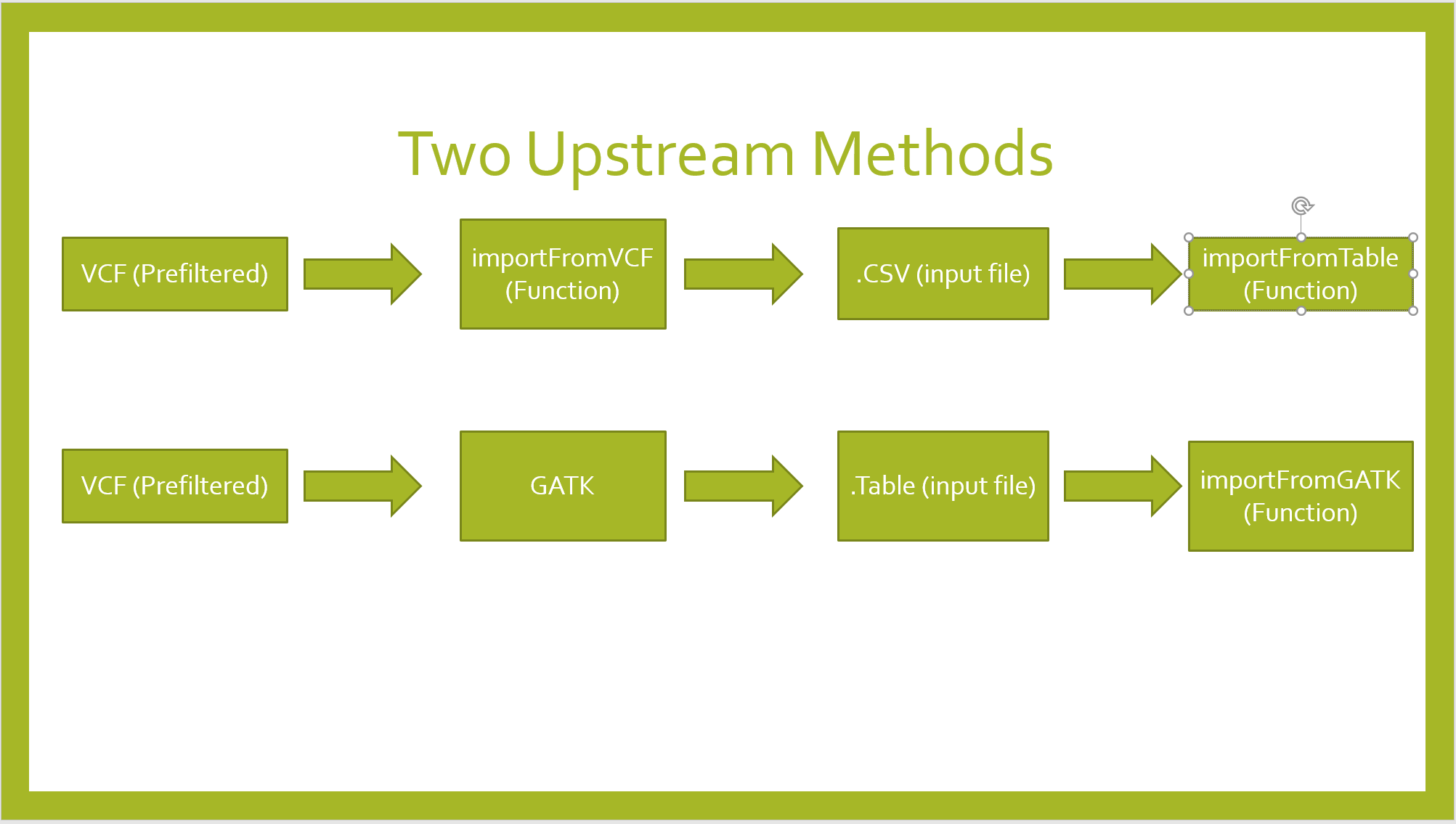
Importing Data
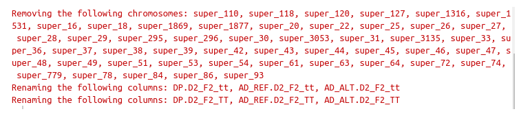
importFromVCF
df <- importFromVCF(file = "freebayes_D2.filtered.vcf", highBulk = "D2_F2_tt", lowBulk = "D2_F2_TT", filname = "Hall")
importFromGATK
An offical Github GATK Genomic Analysis Toolkit repository can be found here to download https://github.com/broadinstitute/gatk
However, we want to clone the repository and make a build:
git clone https://github.com/broadinstitute/gatk


**Navigate to find gradlew and type the command:**
gradlew bundle
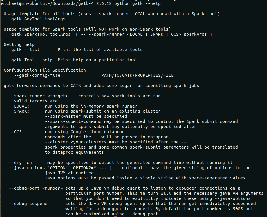
**To verify it is working invoke python interpreter:**
python gatk --help
python gatk --list
*Base Calling:*
*Copy Number Variant Discovery:*
*Coverage Analyis:*
*Diagnostics and Quality Control:*
*Example Tools:*
*Genotyping Arrays Manipulation:*
*Intervals Manipulation:*
*Metagenomics:*
*Methalation-Specific Tools:*
*Other:*
*Read Data Manipulation:*
*Reference:*
*Short Variant Discovery:*
*Structural Variant Discovery:*
*Variant Evaluation and Refinement:*
*Variant Filtering:*
*Variant Manipulation:*
# We are most concerned with Variant Evaluation and Refinement
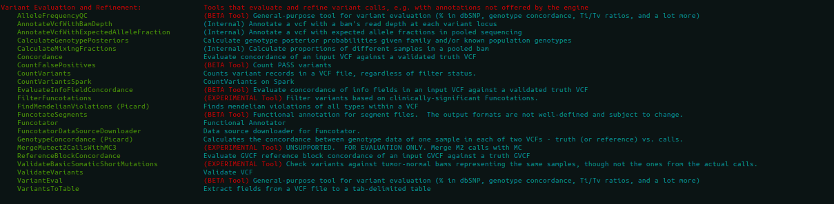
To produce the input file Hall.table, run the following command:
python gatk VariantsToTable --variant freebayes_D2.filtered.vcf --fields CHROM --fields POS --fields REF --fields ALT --genotyp-fields AD --genotype-fields DP --genotype-fields GQ --genotype-fields PL --output Hall.table
Input Fields ImportFromVCF
**Define High bulk and Low bulk sample names as an input object and define parser generated file name. The file name is generated from ImportFromVCF function.**

HighBulk <- "D2_F2_tt"
LowBulk <- "D2_F2_TT"
file <- "Hall.csv"

**Choose and define which chromosomes/contigs will be included in the analysis. The chromosome/contg names are reverse compatible with VCF names.**

Chroms <- c("Chr01","Chr02","Chr03","Chr04","Chr05","Chr06","Chr07","Chr08","Chr09","Chr10")
importFromTable
df <-
  importFromTable(
    file = file,
    highBulk = HighBulk,
    lowBulk = LowBulk,
    chromList = Chroms
  )
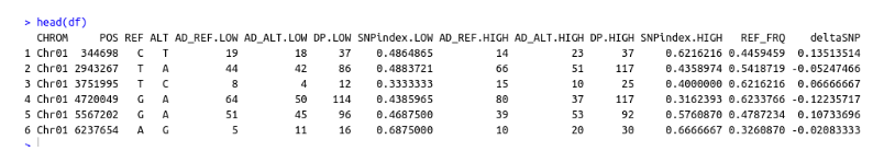
Inspect Header
Input Fields ImportFromGATK
**Define Objects High bulk, Low bulk and file given there proper names.**

HighBulk <- "D2_F2_tt"
LowBulk <- "D2_F2_TT"
file <- "Hall.table"

**Choose which chromosomes/contigs will be included in the analysis.**

Chroms <- c("Chr01","Chr02","Chr03","Chr04","Chr05","Chr06","Chr07","Chr08","Chr09","Chr10")
importFromTable
df <-
  importFromGATK(
    file = file,
    highBulk = HighBulk,
    lowBulk = LowBulk,
    chromList = Chroms
  )
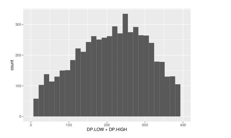
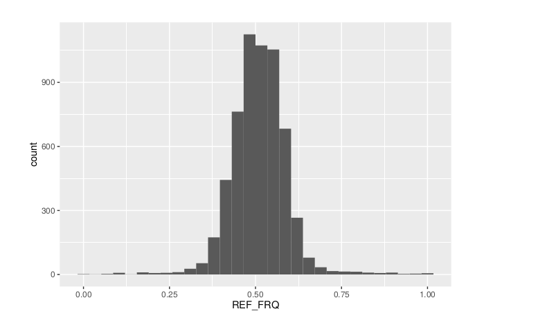
Histograms
**Make histograms associated with filtering arguments. Such as Minimum Depth, Maximum Depth, Reference Allele Frequency, Minimum Sample Depth, and Genotype Quality.

ggplot(data =df) + geom_histogram(aes(x = DP.LOW + DP.HIGH)) + xlim(0,400)


ggsave(filename = "Depth_Histogram.png",plot=last_plot())
ggplot(data = df) + geom_histogram(aes(x = REF_FRQ))
ggsave(filename = "Ref_Freq_Histogram.png",plot = last_plot())
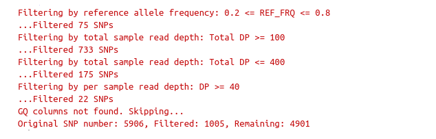
filterSNPs
**Filter SNPs:**
df_filt <- filterSNPs( SNPset = df,
refAlleleFreq = 0.20, minTotalDepth = 100, maxTotalDepth = 400,
minSampleDepth = 40,
minGQ = 0 )
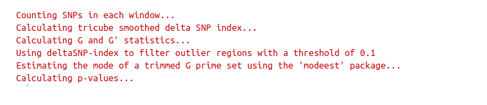
runGprimeAnalysis_MH
**Run G' analysis:**

df_filt<-runGprimeAnalysis_MH(
  SNPset = df_filt,
  windowSize = 5000000,
  outlierFilter = "deltaSNP",
  filterThreshold = 0.1)
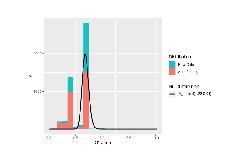
plotGprimeDist_MH
**The plot reveals a skewed G Prime statistic with a really small variance. Perhaps it is due to relatively High Coverage with respect to Bulk Sample Sizes and not a lot of variants called.**

**In addition, Hampels outlier filter in the second argument can also be changed to "deltaSNP".**

plotGprimeDist(SNPset = df_filt, outlierFilter = "Hampel",filterThreshold = 0.1, binwidth = 0.5)
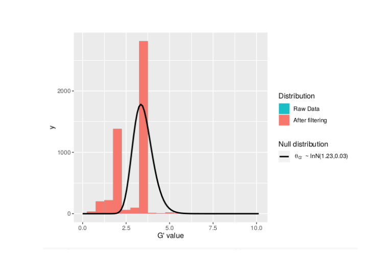
**We can see raw data before and after our filtering step**

plotGprimeDist_MH(SNPset = df_filt, outlierFilter = "deltaSNP",filterThreshold = 0.1,binwidth=0.5)
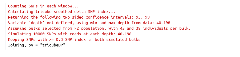
runQTLseqAnalysis_MH
**Run QTLseq analysis:**


df_filt2 <- runQTLseqAnalysis_MH(
  SNPset = df_filt,
  windowSize = 5000000,
  popStruc = "F2",
  bulkSize = c(45, 38),
  replications = 10000,
  intervals = c(95, 99)
)
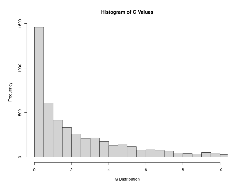
Plot G Statistic Distribution as a Histogram
hist(df_filt2$G,breaks = 950,xlim = c(0,10),xlab = "G Distribution",main = "Histogram of G Values")
plotQTLStats
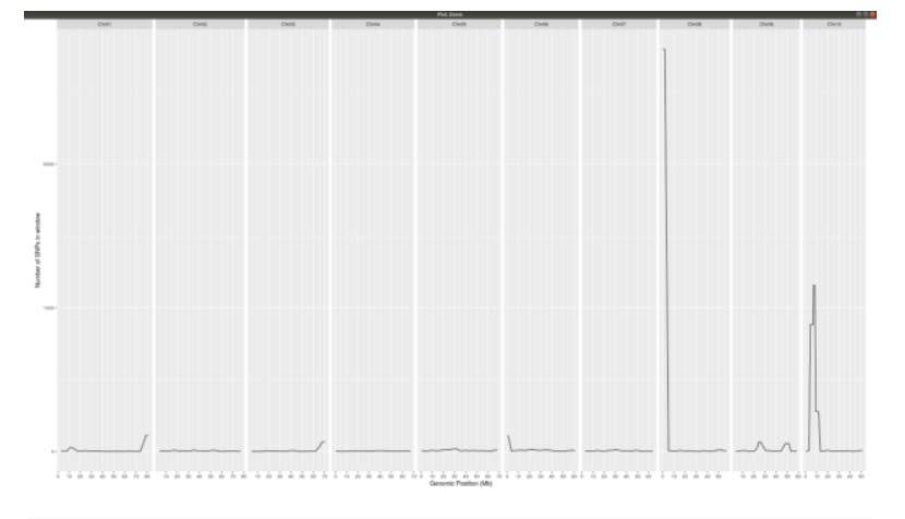
nSNPs
**Plot Snps as a function of chromosome and position values**


plotQTLStats(SNPset = df_filt2, var = "nSNPs")
ggsave(filename = "nSNPs.png",plot = last_plot())
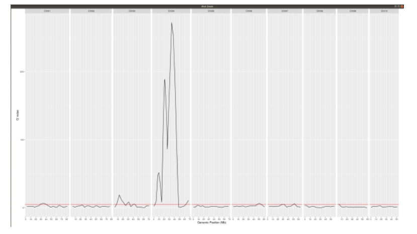
Gprime
**Using QTLStats funciton plot Gprime Statistic with False Discovery Rate Threhshold as a third argument boolean operator as TRUE. The q value is used as FDR threshold null value is 0.05%.**


plotQTLStats(SNPset = df_filt, var = "Gprime", plotThreshold = TRUE, q = 0.01)
ggsave(filename = "GPrime.png",plot = last_plot())
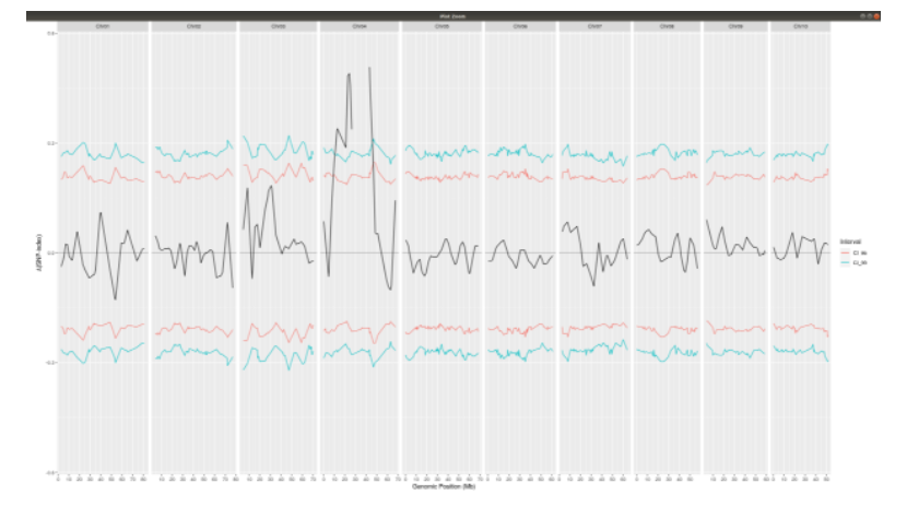
deltaSNP
**Again using plotQTLStats change second argument varaible to deltaSNP and plot.**

plotQTLStats(SNPset = df_filt2, var = "deltaSNP", plotIntervals  = TRUE)
ggsave(filename = "DeltaSNPInterval.png",plot = last_plot())
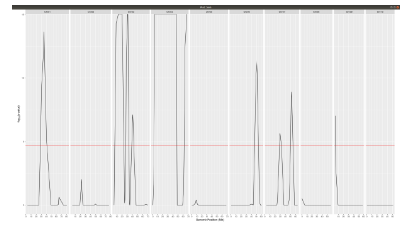
negLog10Pval
**Finally with plotQTLStats plot negLog10Pval.**

plotQTLStats(SNPset = df_filt2, var = "negLog10Pval",plotThreshold = TRUE,q=0.01)
ggsave(filename = "negLog10Pval.png",plot = last_plot())
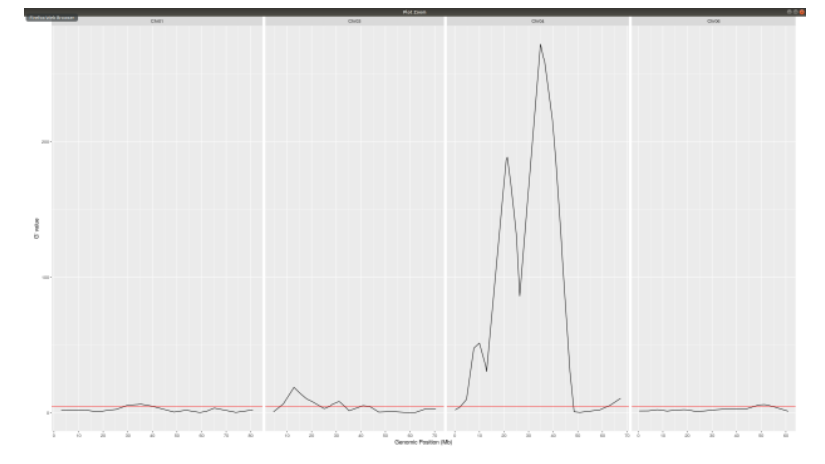
Gprime Subset
**Add subset argument to focus on particular chromosomes one, three, four, and six.**
**The reason is due to signficant QTL regions**


plotQTLStats(SNPset = df_filt2, var = "Gprime",plotThreshold = TRUE,q=0.01,subset = c("Chr01","Chr03","Chr04","Chr06"))
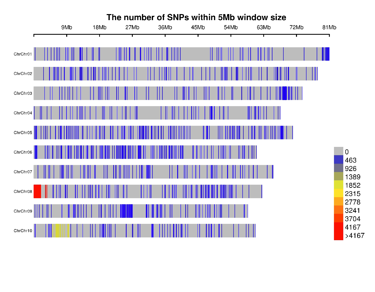
rMVP Package
SNP Densities
install.packages("rMVP")
library(rMVP)
sample<-"Semi_Dwarfism_in_Sorghum"
pathtosample <- "/home/michael/Desktop/QTLseqr/extdata/subset_freebayes_D2.filtered.vcf.gz"
out<- paste0("mvp.",sample,".vcf")
memo<-paste0(sample)
dffile<-paste0("mvp.",sample,".vcf.geno.map")

message("Making MVP data S1")
MVP.Data(fileVCF=pathtosample,
      #filePhe="Phenotype.txt",
      fileKin=FALSE,
      filePC=FALSE,
      out=out)

message("Reading MVP Data S1")
df <- read.table(file = dffile, header=TRUE)
message("Making SNP Density Plots")
MVP.Report.Density(df[,c(1:3)], bin.size = 5000000, col = c("blue", "yellow", "red"), memo = memo, file.type = "jpg", dpi=300)
Export summary CSV
QTLTable(SNPset = df_filt, alpha = 0.01, export = TRUE, fileName = "my_BSA_QTL.csv")
Preview the Summary QTL
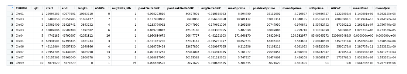
Theory
Contigency Table
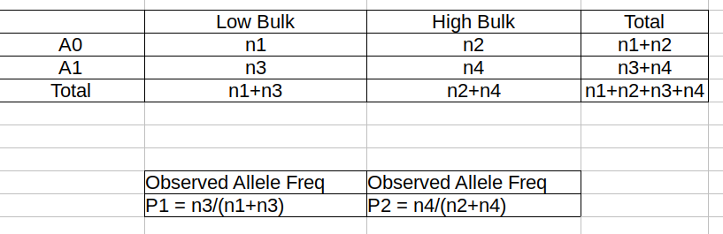
Obs_Allel_Freq
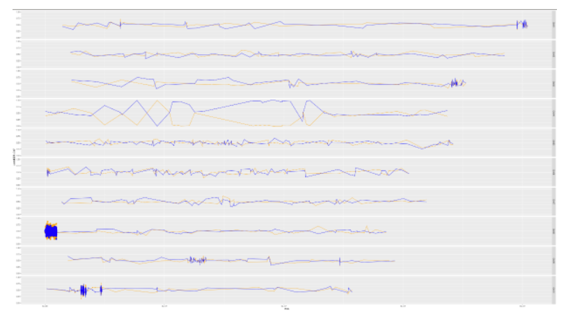
**Use the function to plot allele frequencies per chromosome.**
**Second argument size specifes size of scalar factor on nSNPs and if you have a relatively small SNP set .001 is a good startin point otherwise set to 1**


Obs_Allele_Freq(SNPSet = df_filt, size = .001)
Obs_Allele_Freq2
**Use the function to investigate chromosomal region of interest**

Obs_Allele_Freq2(SNPSet = df_filt, ChromosomeValue = "Chr04", threshold = .90)

Total Coverage and Expected Allelic Frequencies
E(n1) = E(n2) = E(n3) = E(n4) = C/2


**Read in the csv file from High bulk tt**

tt<-read.table(file = "D2_F2_tt.csv",header = TRUE,sep = ",")

**Calculate average Coverage per SNP site**

mean(tt$DP)

**Find REalized frequencies**

p1_STAR <- sum(tt$AD_ALT.) / sum(tt$DP)

**Read in the csv file from Low Bulk TT.**

TT<-read.table(file ="D2_F2_TT.csv",header = TRUE,sep=",")

**Calculate average Coverage per SNP sit**

mean(TT$DP)

**Find Realized frequencies**

p2_STAR <- sum(TT$AD_ALT.) / sum(TT$DP)

**Take the average of the Averages**

C <-(mean(tt$DP)+mean(TT$DP))/2

C<-round(C,0)
**Find Coverage Value**
C
110

E(n1) = E(n2) = E(n3) = E(n4) = C/2 = 55

p2 >> p1 QTL is present
Theory and Analytical Framework of Sampling from BSA
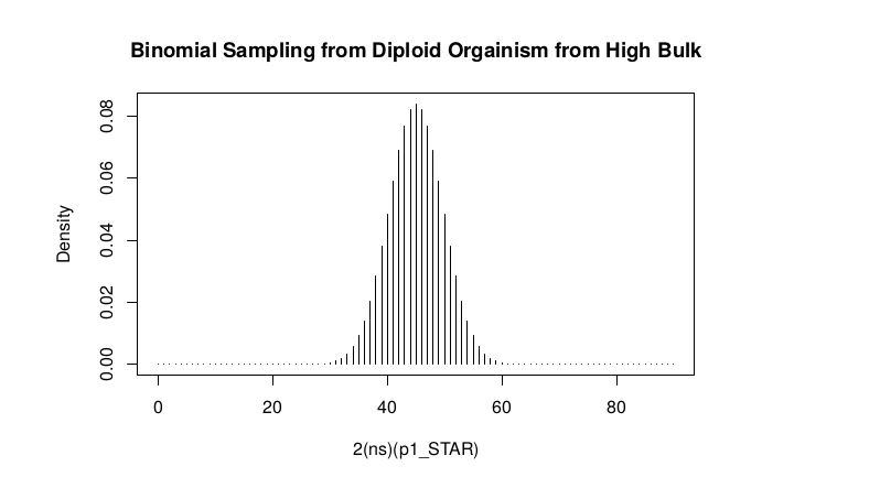
Binomial Sampling
High Bulk
par(mfrow=c(1,1)) Define Ranges of Success success <- 0:90
The Difference between realized and Expected Frequencies
ns : Sample Size taken from Low Bulk
2(ns)p1_star ~ Binomial(2(ns),p1)
p1 Expected Frequencies
Expected Frequencies:
E(n1) = E(n2) = E(n3) = E(n4) = C/2 = 110
We prefer for accuracy and a powerful G Prime Test to have ns >> C >> 1
However, it is not true in this case.
plot(success, dbinom(success, size = 90, prob = .50), type = “h”,main=”Binomial Sampling from Diploid Orgainism from High Bulk”,xlab=”2(ns)(p1_STAR)”,ylab=”Density”)
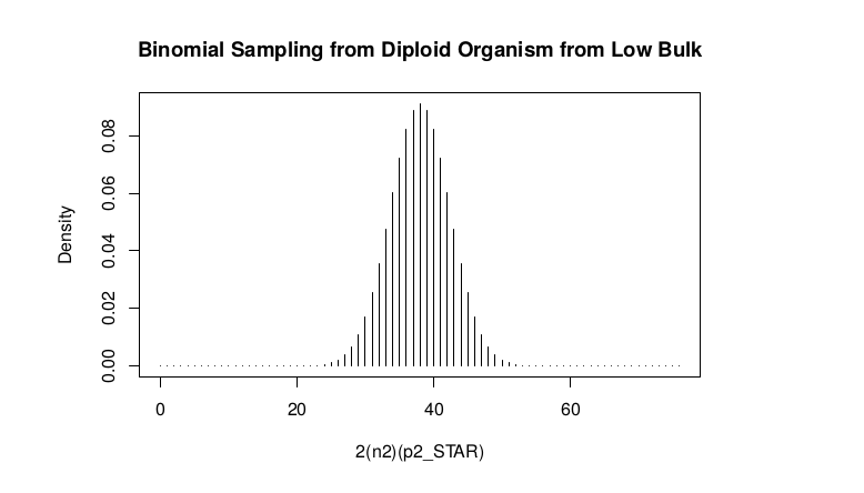
Low Bulk
**ns : Sample Size from High Bulk**
**2(ns)p2_star ~ Binomial(2(ns),p2)**
**p2 Expected Frequencies**
success <- 0:76
plot(success, dbinom(success, size = 76, prob = 0.5), type = "h",main="Binomial Sampling from Diploid Organism from Low Bulk",xlab="2(n2)(p2_STAR)",ylab="Density")
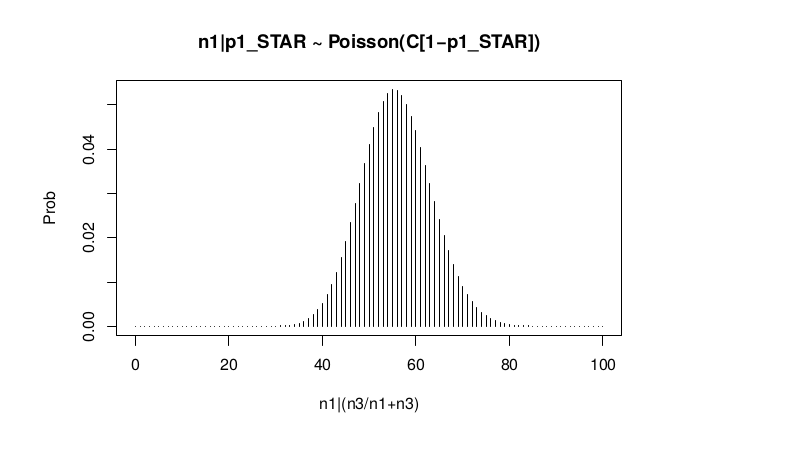
Conditional Distribution of n1 given realized average frequency
par(mfrow=c(1,1))
#Define Ranges of Success (Allele Frequencies High and Low)
success <- 0:100
#n1|p1_star ~ Poisson(lambda)
plot(success, dpois(success, lambda = C*(1-p1_STAR)), type = 'h',main="n1|p1_STAR ~ Poisson(C[1-p1_STAR])",xlab="n1|(n3/n1+n3)",ylab="Prob")
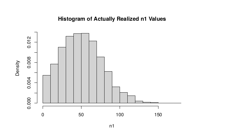
Observed n1
hist(TT$AD_REF., probability = TRUE,main="Histogram of Actually Realized n1 Values",xlab="n1")
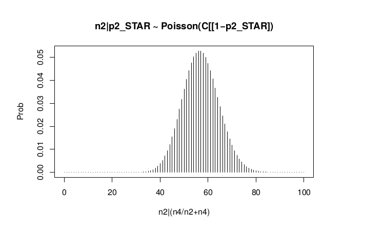
Conditional Distribution of n2 given realized average frequency
#n2|p2_star ~ Poisson(lambda)
plot(success, dpois(success, lambda = C*(1-p2_STAR)), type='h', main="n2|p2_STAR ~ Poisson(C[[1-p2_STAR])",xlab="n2|(n4/n2+n4)",ylab="Prob")
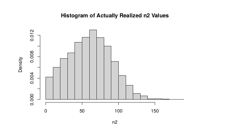
Observed n2
hist(tt$AD_REF., probability = TRUE, main = "Histogram of Actually Realized n2 Values",xlab="n2")
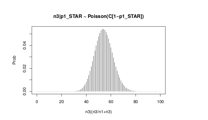
Conditional Distribution of n3 given realized average frequency
#n3|p1_star ~ Poisson(lambda)
plot(success, dpois(success, lambda = C*p1_STAR),type='h',main="n3|p1_STAR ~ Poisson(C[1-p1_STAR])",xlab="n3|(n3/n1+n3)",ylab="Prob")
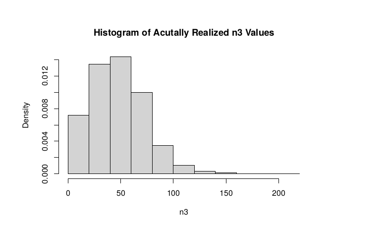
Observed n3
hist(TT$AD_ALT., probability = TRUE, main="Histogram of Acutally Realized n3 Values",xlab="n3")
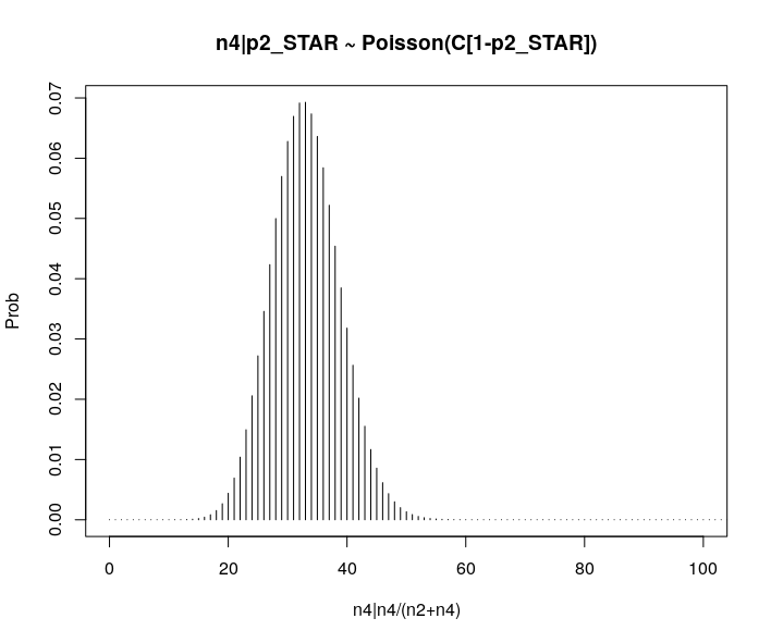
Conditional Distribution of n4 given realized average frequency
#n4|p2_star ~ Poisson(lambda)
plot(success, dpois(success, lambda = C*p2_STAR), type = 'h',main="n4|p2_STAR ~ Poisson(C[1-p2_STAR])",xlab="n4|n4/(n2+n4)",ylab="Prob")
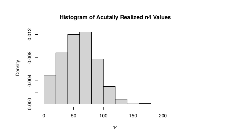
Observed n4
hist(tt$AD_ALT., probability = TRUE, main="Histogram of Acutally Realized n4 Values",xlab="n4")
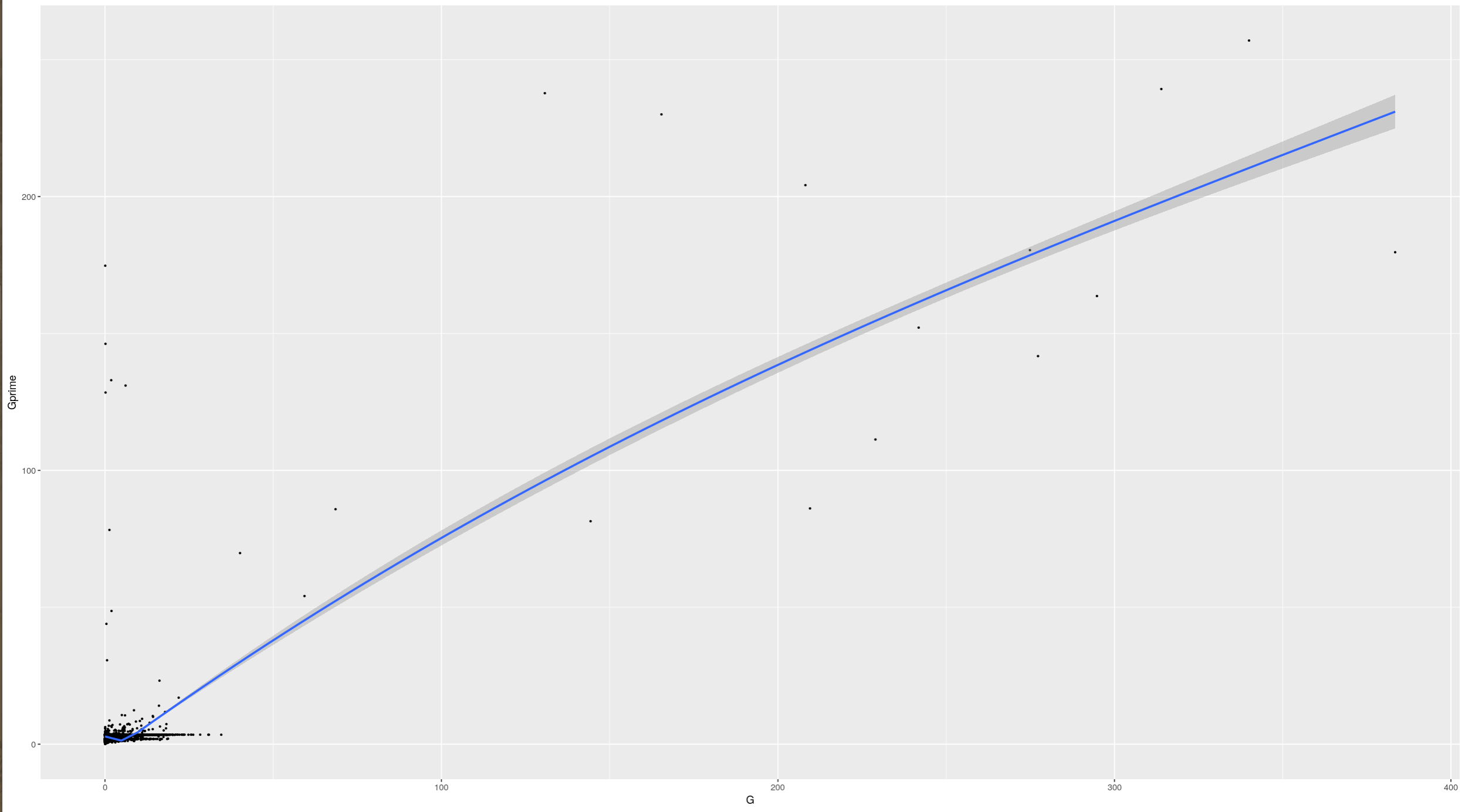
An interdependentaly observed relationship between G and Gprime